As an end of course project in my introductory data science course, I worked with a team of three classmates to see with what accuracy we could predict the pricing of Airbnb rentals in Seattle given some data about a particular listing. This research was primarily motivated by the similarity of this problem to a classical use case of machine learning: house price prediction. As a regular user of the Airbnb service I was interested in the relationships between certain features of a listing and the resulting price. As a resident of Seattle I was also curious to see if the listing price in select areas of the city was consistent with my own perception of an area's value.
Choosing The Dataset
As alluded to above, I chose this dataset because I knew I would be able to make use of a number of machine learning regression algorithms to help me predict the price of Airbnb listings. After trawling through the datasets that Kaggle had to offer, I settled on thishttps:www.kaggle.comairbnbseattlelistings.csv one. It included an impressive amount of features related to each property as well as metadata about the host. All of this data was obtained through an extensive web scrape of the Airbnb site. Besides the quantity of features available, the data was generally well formatted and reasonably clean. This cut down on the data cleaning work the needed to be done prior to beginning the analysis.
Exploring And Cleaning The Data
Even with a relatively clean dataset such as this one, there was still a substantial amount of work to be done to prepare the data for analysis. I was able to reduce the number of listings features from 92 to 81 by just dropping all features that only contained one unique value. From there I performed an exploratory data analysis to determine what features I wanted to be considering for my models. By running several multivariate linear regressions with price as the dependent variable, I was able to get a better idea of what features had some type of relationship with listing price.
Based on the relationships seen in the linear regression and my own intuitions about the problem I selected 19 features to be used in the models. After selecting these features I was able to finish up the data cleaning process, handling missing values by employing a variety of methods based on the sparsity of a particular tuple or feature. For instance, to populate the missing listing review scores I used the median value of the scores and the pandas fillna() function.
# populate review NA's with median
pd.options.mode.chained_assignment = None
df['review_scores_rating'] = df.review_scores_rating.fillna(df.review_scores_rating.median())
Because some significant features were categorical variables with a large number of values, I needed to convert them to dummy variables so that they could be used in a regression. This became an issue because of the quantity of unique categories that some features contained. When converting to dummy variables using all those categories I was left with a dataframe with hundreds of features. This type of problem was most severe for the neighborhood and property type features. I solved this by filtering the property types to only include the top 6 most common and changing the scope of the neighborhood feature to use the generalized neighborhood zones like Capitol Hill and University District. The methods I used to clean the data can be viewed in their entirety within this python jupyter notebook.
Adding Additional Features
I was also interested to see if the description the listing written by the host had an impact on the price of that listing. More specifically, I wanted to see if the textual sentiment of the listing description had an effect on the price. To add this feature to the dataset we used the Microsoft Azure Text Sentiment Analysis API with Postman requests to send the text of each description to Microsoft for sentiment analysis. With these requests we assigned a sentiment value on a scale of 1 - 100 of the listing description to each listing in the dataset.
More Exploration
As a baseline for feature performance I performed a basic ordinary least squares regression, predicting price using the handful of variables that had previously performed well in the data cleaning process.
formula = 'price ~ SELECT_FEATURES‘
mod1 = smf.ols(formula=formula, data=airbnb_data_dummies).fit()
mod1.summary()
Overall, the regression had an R-squared of .581, indicating that the variables used at least explain the majority of variation in listing pricing. Unsurprisingly, features like bathrooms, bedrooms, and number of guests the listing can accommodate have strong positive relationships with price.
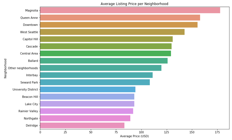
I also took a look at the relationship between the neighborhood of a listing and the average price of a listing in that neighborhood.
Using the sentiment score, we visualized the positivity of language in the listing description against price.
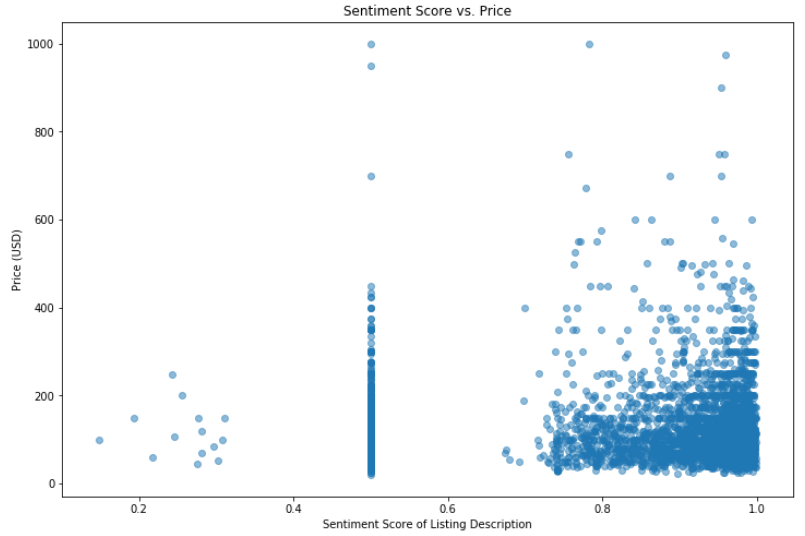
It is interesting to note that the few listings that had low sentiment had generally lower prices. Most tended to have high sentiment, which was expected as the descriptions are intended to sell the home. The clustering of listings at the 0.5 score mark is an artifact of the sentiment classifier used text blobs that are neutral or cannot be classified are given scores of 0.5.
Predicting Price Using Machine Learning
To predict the price of a listing I used the process of splitting our data into train and test sets, building data pipelines, and predicting using various machine learning algorithms. All the algorithms I used were from the popular sklearn package.
# split into train and test
train_features, test_features, train_outcome, test_outcome = train_test_split(
    airbnb_data_dummies.drop("price", axis=1),
    airbnb_data_dummies.price,
    test_size=0.20
)
In order to determine the best hyperparameters for each model I used sklearns grid search for model optimization. I tested three common machine learning algorithms to see which ones performed the best on my data k-nearest neighbor, random forest, and a neural network. An example of the pipeline using the neural network looks like this:
nn_pipeline = make_pipeline(
    MinMaxScaler(),
    PolynomialFeatures(1),
    MLPRegressor()
)
nn_param_grid = {
   'mlpregressor__learning_rate':["constant", "invscaling", "adaptive"],
    'mlpregressor__solver':["lbfgs", "sgd", "adam"],
    'mlpregressor__activation':["relu"]
}
nn_grid = GridSearchCV(nn_pipeline, nn_param_grid, cv=3, scoring="neg_mean_absolute_error")
nn_grid.fit(train_features, train_outcome)
nn_grid.score(test_features, test_outcome)
After rigorously testing all the models defined above, the model that consistently performed the best was the multi-layer perceptron neural net. Out of the three, k nearest neighbor typically reported mean absolute errors in the 38-35 range, random forest reported mean absolute errors in the 37-34 range, and the neural network scored in the 35-31 range. Comparing the spread of each model's errors against the test data confirms the neural network as the most accurate of the three.
Assessing Model Performance
As a way to determine accuracy of the models we plotted the predicted values against the true values.
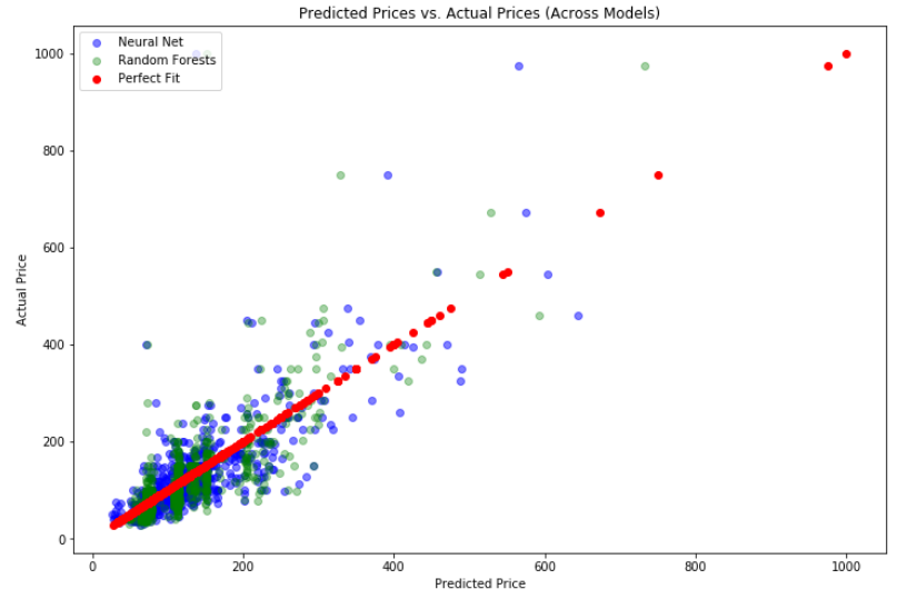
The resulting plot has the predictions of the two models on a slope generally conforming to xy, indicating relatively accurate predictions. In order to visualize the prediction error across models we compared the performance of the neural network to the random forest model.
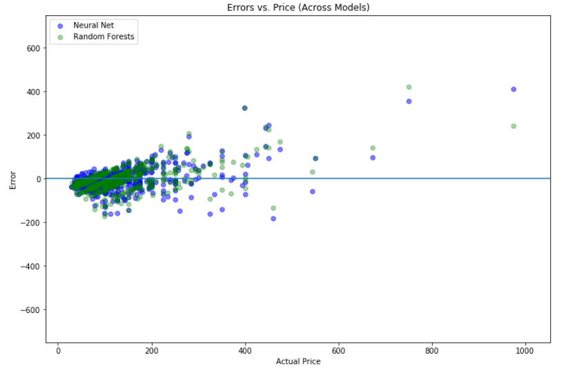
Both models seem to mispredict similar listings. These missed predictions are generally the outliers in the dataset. You often see pairs of blue and green dots together, indicating that listings that one model mispredicts, the other model is likely to mispredict as well. There also appear to be claw-like streaks produced by the Random Forest regressor, mirroring the linear patterns in the previous visualization. As a final model performance visualization I made a violin plot to compare the errors for the Neural Net across all property types, to see if we were better or worse at predicting specific properties.
# get errors for the neural network
nn_errors =  pd.DataFrame(test_outcome - nn_grid.predict(test_features))
nn_errors.rename({"price": "error"}, axis='columns', inplace=True)

# fix indexes
nn_errors.index = nn_errors.index.astype(str)
property_errors.index = property_errors.index.astype(str)
res = nn_errors.join(property_errors)
res.error = res.error.abs()

violin_plot = sns.violinplot(x="property_type", y="error", data=res)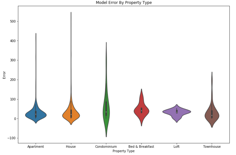
Apartments, houses, and townhouses appear to have the lowest errors, potentially due to a higher number of listings. However, we also observe huge spikes in error in these property types, especially houses, likely due to outliers on the extremely expensive end. Intuitively, the extremely expensive Airbnb's will likely be large homes and perhaps condominiums, so these naturally will have more extreme high-end outliers.
Conclusions
It turns out that given a set of features and a sufficient amount of data, you can use machine learning to predict somewhat accurately the listing price of an Airbnb in Seattle While the work done on this project was by no means groundbreaking technically, it was a great way for me to use my data science abilities in approaching a problem that would be difficult to solve without using these tools. Reflecting back on the work I did, I'm excited to use the skills I learned in this project to ask and answer future questions.
Project Resources
I've published the code used for this project on GitHub here. You can read the full paper I co-authored about this work here.